Anomoly Dectection 顾名思义“异常识别”,给定一个 dataset(with features),训练出一种模型,当出现新数据时,判断该数据是否正常。
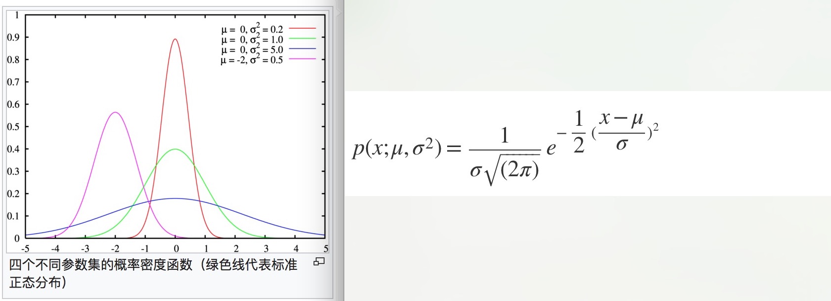
首先我们先来简单聊下高斯分布 Gaussian Distribution(正态分布 Normal Distribution),我们认为中间状态是事物的常态,过高和过低都属于少数。高斯分布的概率密度函数曲线呈钟形,因此人们又经常称之为钟形曲线。高斯分布的概率密度函数为:
 所以识别异常值的过程就变为求解概率的数学问题,当概率值低于某个阈值 ϵ ,即 p(x) < ϵ 时,我们把它认为是异常值。
Anomoly Dectection Original Model
Algorithm
应用于实际例子中,给定训练集 {x1, … ,xm},其中每个 x 是一个 n 维向量(n 个 features)。那么 x 为正常值的概率为每一个单独特征为正常值的概率的乘积:

Features Transform
在异常识别中,feature 是一个算法好坏的重要因素,但是有些 feature 的分布不满足高斯分布,这时我们就需要进行 features transform.
![]() 检查转换完的 feature 是否满足高斯分布图
检查转换完的 feature 是否满足高斯分布图
Developing and Evaluating an Anomaly Detection System
之前我们讨论概率密度函数时,没有用到 y 值,即把所有的 training data 当作 unlabled data 来用。但是如何评估算法的好坏呢?
- 标记数据,区分中正常数据和异常数据
- 将数据集按 60(training) : 20(cv):20(test) 来拆分,其中 training data 全部为正常数据,而将异常数据平均分配到 cv & test 中
- 用全部为正常数据的 training data 来求解 μ 和 σ2

Anomaly Detection vs. Supervised Learning
经过上面的描述,是不是有一种感觉,Anomaly Detection 和 Supervised Learning 中的分类问题很像?的确是这样的,两者的目的一样,但应用场景不同: Use anomaly detection when…
- We have a very small number of positive examples (y=1 … 0-20 examples is common) and a large number of negative (y=0) examples.
- We have many different “types” of anomalies and it is hard for any algorithm to learn from positive examples what the anomalies look like; future anomalies may look nothing like any of the anomalous examples we’ve seen so far.
Use supervised learning when…
- We have a large number of both positive and negative examples. In other words, the training set is more evenly divided into classes.
- We have enough positive examples for the algorithm to get a sense of what new positives examples look like. The future positive examples are likely similar to the ones in the training set.
Multivariate Gaussian Distribution
之前提到的异常识别算法在某种情况下会出错,如:
 图中用绿色标记出来的数据是一个异常数据(离别的正常数据很远),但是它的两个 features 分布都在正常范围内,通过之前讨论的算法是无法捕捉这种情况的:即 features 之间有相互关系,本图中的两个特征是一同递增/递减。
所以我们引入了一种优化算法:Multivariate Gaussian Distribution(多元高斯分布)。这种算法不是把 n 维 features 独立计算概率值再相乘,而是把所有特征当成一个整体,可以自动捕捉到不同 features 之间的关系,并用一个统一的公式计算:

 其中,μ ∈ ℝn , Σ ∈ ℝn×n
该公式的等高热度图为:
其中,μ ∈ ℝn , Σ ∈ ℝn×n
该公式的等高热度图为:


Make a Choose between Original Model and Multivariate Gaussian Distribution
原始模型可以当做多元高斯分布的一个特例,即特征之间没有相互关联,反应到数学公式上:Σ 是一个对角矩阵(即除对角线外,矩阵的其他元素全部为 0)。

其实为了解决原始模型无法顾及 features 间关联的问题,可以通过添加 feature 来解决。之前我们提到,计算机的 CPU load 和 memory 本质上有正相关性,虽然单独计算两个 features 无法体现出相关性来,但是我们可以添加 x3 = CPU load / memory 这个新 feature 来反映这种关联性。
由于算法复杂度的原因,不同的场景可以选择不同的算法来执行:
| original model | Multivariate Gaussian Distribution |
|---|---|
| 需要手动创建 feature 捕获特征关系 | 自动捕捉特征关联关系 |
| 计算速度更快 | 计算速度慢 |
| 适合 training data 比较小的情况 | 适合 training data 远远大于 features 的情况 |